
Next part of our ‘the overfitting trap’ series… Today, we are going to see the impact of different parameters, regularization techniques and ensemble methods on the overfitting problem.
Before delving into our topic, let’s talk about again ‘what is overfitting’. It is something that happens when a machine learning model learns the training data too well, memorizing it instead of generalizing to new data. It performs great on the training data, but poorly on unseen data.
As you can understand, it is something that we need to avoid. For this, we can take some precautions. In the fourth topic of this problem, we will see how can we solve that problem with different parameters, different regularization techniques and the recommended solution of ensemble methods.
Different Parameters
Every machine learning model has its own parameters. You can specialize your model with these parameters. While the accuracy score of the model can often be increased with this process, sometimes the accuracy score of the overfitted model can be reduced and made smooth.
For instance, think about Decision Tree model. It is something that can over-learn, because their learning process is greedy.
So, what we do here is create a model with Python 3.10. Firstly, let me show you a Python codes for the model in my idea.
# required imports
from sklearn.tree import DecisionTreeClassifier
from sklearn.metrics import accuracy_score

# create the decision tree classifier model
dt_model = DecisionTreeClassifier(
    max_depth=3,
    min_samples_split=5,
    min_samples_leaf=2,
    max_features='sqrt'
)

# train the model
dt_model.fit(X_train, y_train)

# make the predictions on the test dataset
y_pred = dt_model.predict(X_test)

# evaluate the model
accuracy = accuracy_score(y_test, y_pred)
print(f"Accuracy of the model: {accuracy}")
If we think about the example above, we can say the following about the parameters in it:
- Max_depth: Limits maximum depth of the tree. For example, the decision tree here can reach a maximum of 3 levels deep.
- Min_samples_split: Minimum required number of samples that splits a node. Here, we need 5 samples to split a node.
- Min_samples_leaf: Minimum required number of samples that need to be found in each leaf node. For here, it is just 2 samples.
- Max_features: Limits the maximum number of features to be considered in each split (for here, it is square root of the features).
So, we limited the learning process of our model. Click here, if you want to see more parameters.
Actually, we have to the best parameters for our model to reduce risk of the overfitting -also we have to improve the accuracy. For this, we need to try parameters. Another way for this is GridSearchCV, which is something I told you in this article.
Regularization Techniques
It is another good technique to reduce our model’s overfitting risk. We can talk about two techniques in this part. One of them is L1 regularization (Lasso), another one is L2 regularization (Ridge).
These two has the same purpose: reduce risk of the overfitting. They are working with adding a penalty to a loss function that aims changing the direction of regression curve.
Let’s talk about formulas of these regressions. For Lasso (L1):

And for Ridge (L2):

•  : i. observation of dependent variable
•
: i. observation of dependent variable
•  : i. observation of j. independent variable
•
: i. observation of j. independent variable
•  : intercept
•
: intercept
•  : coefficient of the jth independent variable
•
: coefficient of the jth independent variable
•  : number of observations
•
: number of observations
•  : number of independent variables
•
: number of independent variables
•  : regularization parameter
As you can see above, formulas of Lasso and Ridge is almostly the same. Both of them add a penalty to the loss function. The only difference between them is Ridge has squared beta value in its formula.
So we can change the shape of the regression line with these methods. Let’s see a graph with/without regularization below.
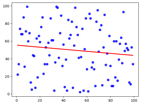
Image 1 shows a graph without regularization. Now, see the Image 2 -a graph with regularization.
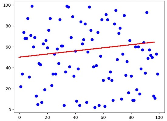
You have seen that applying regularization can thus change the shape of the graph. This reduces the risk of overfitting by changing the regression line.
To end this section, let’s talk about sample Lasso and Ridge regression creation codes (variables starting with y_pred_ are the y variables we have newly created after the regression). For Lasso:
# import lasso
from sklearn.linear_model import Lasso

# create lasso regression model
lasso_model = Lasso(alpha=1.0)
lasso_model.fit(x, y)

# make predictions
y_pred_lasso = lasso_model.predict(x)
For Ridge:
# import ridge
from sklearn.linear_model import Ridge

# create ridge regression model
ridge_model = Ridge(alpha=10.0)
ridge_model.fit(x, y)

# make predictions
y_pred_ridge = ridge_model.predict(x)
So, that’s it. You can use these codes to use what I told you in this section. Let’s continue to the last part of this article.
Ensemble Methods
Our last topic is Ensemble Methods. This in machine learning combine multiple models to make a better prediction than any single model could achieve alone. It’s like getting a group of experts to vote on a decision, improving accuracy and robustness.
Here, something called Majority Vote takes place. For example, we bring lots of Decision Tree together, and give them a data to predict its independent variable. After that, lots of Decision Tree predict what is our data’s class, and we take average of them.
For example, if most of Decision Trees say ‘1’, then our class will be predicted like ‘1’. In the same way, we may see ‘0’ output.
In here, I will show you 2 kind of Ensemble Methods:
- Random Forest: It is a machine learning algorithm that works by averaging the predictions of many individual trees, each trained on a different random subset of the data.
- AdaBoost (Adaptive Boosting): It is a machine learning algorithm that combines multiple weak learners (like decision trees) into a strong learner. It works by iteratively weighting the training samples, giving more importance to misclassified ones, and then training a new weak learner on the weighted data. This process repeats until a desired accuracy is achieved, resulting in a model that is more robust to noise and outliers.
They are wonderful techniques and generally they give better accuracies then Decision Tree model. Let me show you code examples of them. For Random Forest:
# import random forest classifier
from sklearn.ensemble import RandomForestClassifier

# create a random forest model
rf_classifier = RandomForestClassifier(n_estimators=100)

# train the model
rf_classifier.fit(X_train, y_train)

# make predictions with the model
y_pred = rf_classifier.predict(X_test)
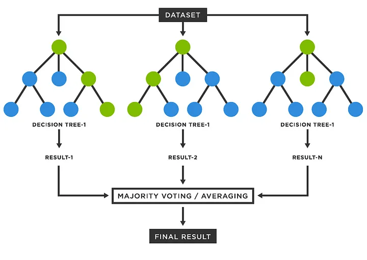
As you can see in the code, we generated our Random Forest Classifier model. It is a forest with Decision Trees and it predicts with average of them. For AdaBoost:
# import adaboost classifier and decision tree classifier
from sklearn.ensemble import AdaBoostClassifier
from sklearn.tree import DecisionTreeClassifier

# create a decision tree model for base
dtc = DecisionTreeClassifier(max_depth=1)

# create an adaboost model
ada = AdaBoostClassifier(base_estimator=dtc, n_estimators=100)

# train the model
ada.fit(X, y)

# Make predictions on new data
predictions = ada.predict(new_data)
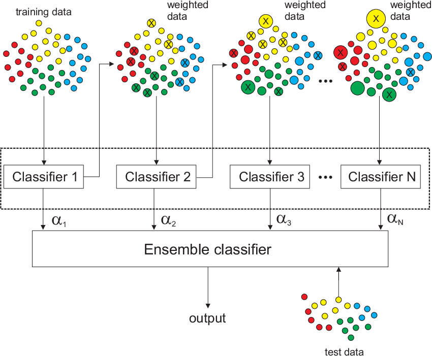
As you can see in the code, we created our base estimator with Decision Tree, so AdaBoost works with Decision Trees right now -as we wanted. Both of these can reduce risk of the overfitting right now.
Thus, I have shown you a few models that you can use directly instead of the Decision Tree. You can use all of the techniques in this article to avoid from overfitting.
Thank you for reding this part of post. Return the main article by clicking here.
Bibliography
Günay, D.. Random Forest. Medium. https://medium.com/@denizgunay/random-forest-af5bde5d7e1e
Jorge Pérez-Aracil. Diagram of the AdaBoost algorithm exemplified for multi-class classification problems. ResearchGate. https://www.researchgate.net/figure/Diagram-of-the-AdaBoost-algorithm-exemplified-for-multi-class-classification-problems_fig2_362065998

Leave a comment